BlackBody

class jdaviz.models.physical_models.BlackBody(*args, **kwargs)

Bases: Fittable1DModel

Blackbody model using the Planck function.

Parameters:

temperatureQuantity [‘temperature’]

Blackbody temperature.

scalefloat or Quantity [‘dimensionless’]

Scale factor

output_units: `~astropy.units.CompositeUnit` or string

Desired output units when evaluating. If a unit object, must be equivalent to one of erg / (cm ** 2 * s * Hz * sr) or erg / (cm ** 2 * s * AA * sr) for surface brightness or erg / (cm ** 2 * s * Hz) or erg / (cm ** 2 * s * AA) for flux density (in which case the pi is included internally and should not be passed in scale - see notes below). If a string, can be one of ‘SNU’, ‘SLAM’, ‘FNU’, ‘FLAM’ which reference the units above, respectively.

Notes

Model formula:

\[B_{\nu}(T) = A \frac{2 h \nu^{3} / c^{2}}{exp(h \nu / k T) - 1}\]

Deprecated support for non-dimensionless units in scale:

If scale is passed with non-dimensionless units that are equivalent to one of the supported output_units, the unit is stripped and interpreted as output_units and the float value will account for the scale between the passed units and native output_units. If scale includes flux units, the value will be divided by pi (since solid angle is included in the units), and re-added internally when returning results. Note that this can result in ambiguous and unexpected results. To avoid confusion, pass unitless scale and output_units separately.

Examples

>>> from astropy.modeling import models
>>> from astropy import units as u
>>> bb = models.BlackBody(temperature=5000*u.K)
>>> bb(6000 * u.AA)  
<Quantity 1.53254685e-05 erg / (cm2 Hz s sr)>

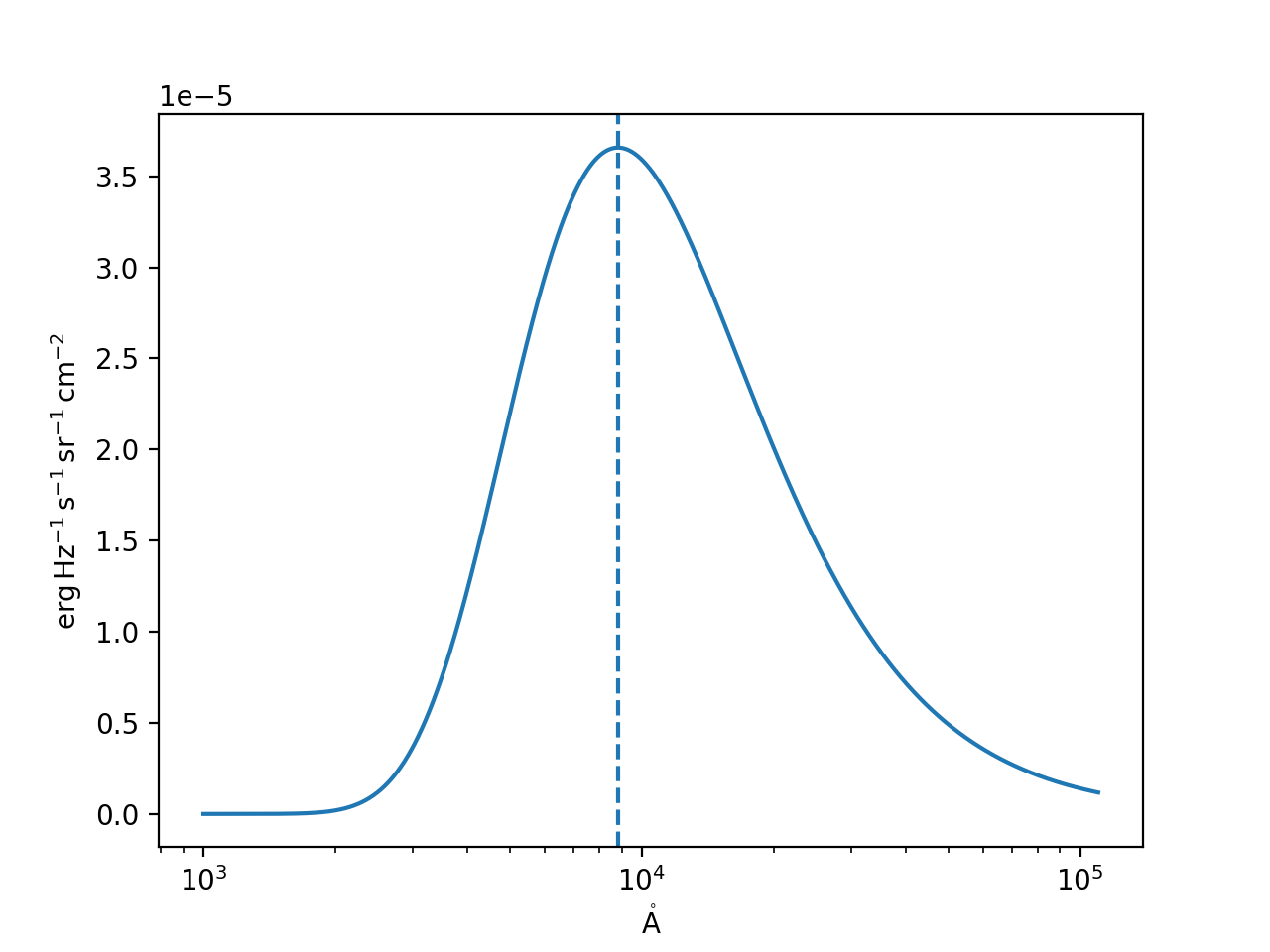
import numpy as np
import matplotlib.pyplot as plt

from astropy.modeling.models import BlackBody
from astropy import units as u
from astropy.visualization import quantity_support

bb = BlackBody(temperature=5778*u.K)
wav = np.arange(1000, 110000) * u.AA
flux = bb(wav)

with quantity_support():
    plt.figure()
    plt.semilogx(wav, flux)
    plt.axvline(bb.nu_max.to_value(u.AA, equivalencies=u.spectral()), ls='--')
    plt.show()

(Source code, png, hires.png, pdf)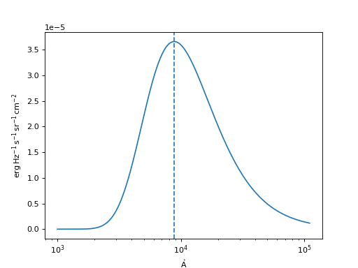

Attributes Summary

bolometric_flux	Bolometric flux.
input_units	This property is used to indicate what units or sets of units the evaluate method expects, and returns a dictionary mapping inputs to units (or None if any units are accepted).
input_units_equivalencies
lambda_max	Peak wavelength when the curve is expressed as power density.
nu_max	Peak frequency when the curve is expressed as power density.
output_units	Return a dictionary of output units for this model given a dictionary of fitting inputs and outputs.
param_names	Names of the parameters that describe models of this type.
scale
temperature

Methods Summary

evaluate(x, temperature, scale)

Evaluate the model.

Attributes Documentation

bolometric_flux

Bolometric flux.

input_units

input_units_equivalencies = {'x': [(Unit("m"), Unit("Hz"), <function spectral.<locals>.<lambda>>), (Unit("m"), Unit("J"), <function spectral.<locals>.<lambda>>), (Unit("Hz"), Unit("J"), <function spectral.<locals>.<lambda>>, <function spectral.<locals>.<lambda>>), (Unit("m"), Unit("1 / m"), <function spectral.<locals>.<lambda>>), (Unit("Hz"), Unit("1 / m"), <function spectral.<locals>.<lambda>>, <function spectral.<locals>.<lambda>>), (Unit("J"), Unit("1 / m"), <function spectral.<locals>.<lambda>>, <function spectral.<locals>.<lambda>>), (Unit("1 / m"), Unit("rad / m"), <function spectral.<locals>.<lambda>>, <function spectral.<locals>.<lambda>>), (Unit("m"), Unit("rad / m"), <function spectral.<locals>.<lambda>>), (Unit("Hz"), Unit("rad / m"), <function spectral.<locals>.<lambda>>, <function spectral.<locals>.<lambda>>), (Unit("J"), Unit("rad / m"), <function spectral.<locals>.<lambda>>, <function spectral.<locals>.<lambda>>)]}

lambda_max

Peak wavelength when the curve is expressed as power density.

nu_max

Peak frequency when the curve is expressed as power density.

output_units

param_names = ('temperature', 'scale')

Names of the parameters that describe models of this type.

The parameters in this tuple are in the same order they should be passed in when initializing a model of a specific type. Some types of models, such as polynomial models, have a different number of parameters depending on some other property of the model, such as the degree.

When defining a custom model class the value of this attribute is automatically set by the Parameter attributes defined in the class body.

scale = Parameter('scale', value=1.0, bounds=(0, None))

temperature = Parameter('temperature', value=5000.0, unit=K, bounds=(0, None))

Methods Documentation

evaluate(x, temperature, scale)

Evaluate the model.

Parameters:

xfloat, ndarray, or Quantity [‘frequency’]

Frequency at which to compute the blackbody. If no units are given, this defaults to Hz.

temperaturefloat, ndarray, or Quantity

Temperature of the blackbody. If no units are given, this defaults to Kelvin.

scalefloat, ndarray, or Quantity [‘dimensionless’]

Desired scale for the blackbody.

Returns:

ynumber or ndarray

Blackbody spectrum. The units are determined from the units of scale.

Note

Use numpy.errstate to suppress Numpy warnings, if desired.

Warning

Output values might contain nan and inf.

Raises:

ValueError

Invalid temperature.

ZeroDivisionError

Wavelength is zero (when converting to frequency).