Data Analysis Plugins
The Cubeviz data analysis plugins include operations on both Spectrum1D one dimensional datasets and SpectralCube objects. Plugins that are specific to 1D spectra are described in more detail under Specviz:Data Analysis Plugins. All plugins are accessed via the plugin icon in the upper right corner of the Cubeviz application.
Gaussian Smooth
Gaussian smoothing can be applied either to the spectral or spatial dimensions of a cube. Spectral smoothing is described in more detail under Specviz:Data Analysis Plugins:Gaussian Smoothing.
See also
- Gaussian Smooth
Specviz documentation on gaussian smoothing of 1D spectra.
Collapse
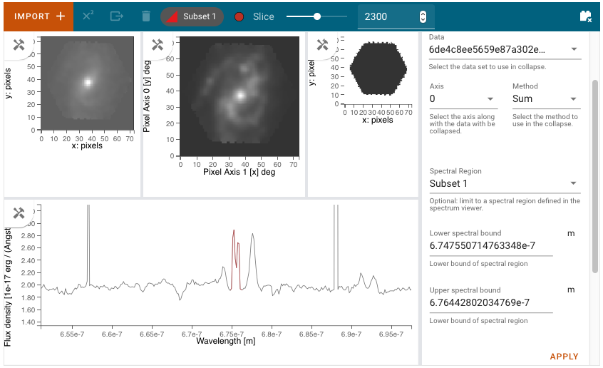
The Collapse plugin collapses a spectral cube along any one axis (x, y , or wavelength) to create a 2D image. For spatial axes, the full extent of the selected dimension is included in the collapse. For the spectral axis, a wavelength range for collapse can be specified using a spectral subset or by entering the wavelength range manually.
To make a 2D image, first go to the Collapse plugin and select the cube dataset using the Data pulldown. Then set the Axis to the dimension to be collapsed (0, 1, or 2). Next, select the method for collapse (Mean, Median, Min, Max, or Sum) in the Method pulldown. To collapse a limited spectral subregion, you can either create and select a Region in the spectrum viewer, or enter the lower and upper spectral bounds manually. When you APPLY the Collapse, a 2D image is created. You can load this into any image viewer pane to inspect the result. For example, the Collapse Sum over an emission line is shown in the middle image viewer of the above figure.
Model Fitting
The Model Fitting plugin is described in more detail by the Specviz:Data Analysis Plugins:Model Fitting documentation. For Cubeviz, there is an additional option to fit the model over each individual spaxel by pressing Apply to Cube. The fit parameter planes are saved in a data structure that can be accessed in a jupyter notebook. The best model fit, evaluated over the cube is also saved to a dataset with the label specified in the Model Label field (default ‘Model’).
See also
- Model Fitting
Specviz documentation on fitting spectral models.
Contours
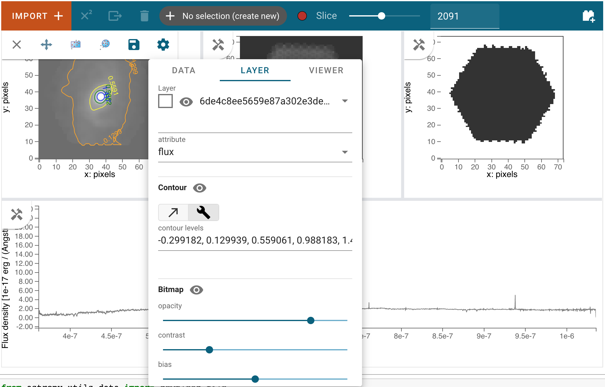
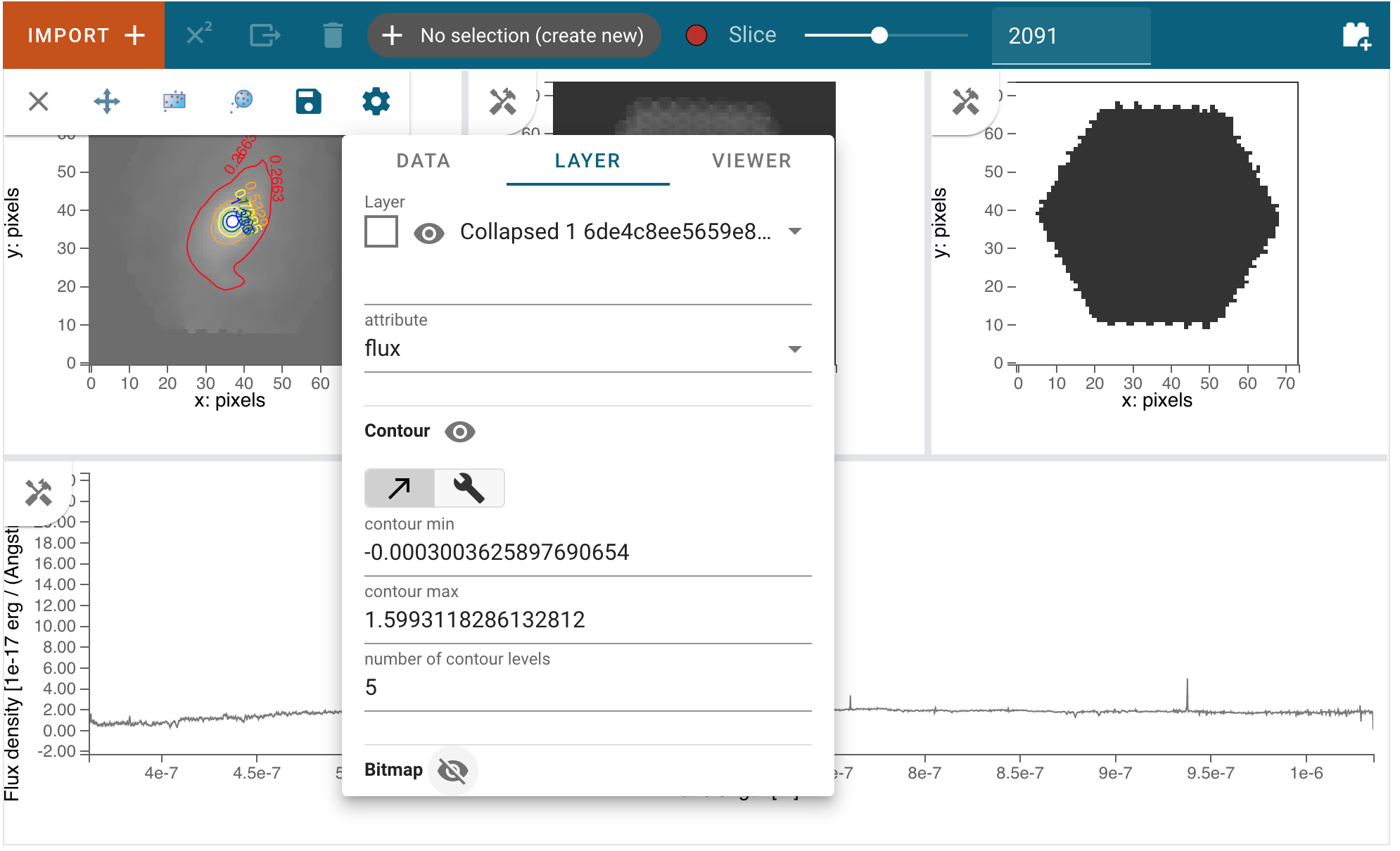
Contours of an image can be generated and overplotted on that image. Go to the Layer tab in the image viewer settings window. To activate Contours, click on the Eye with a cross icon and choose either the Linear icon for auto-contours or the Custom icon to set your own levels. The specified levels will appear as labeled, color-coded contours in the image viewer, on top of the image.
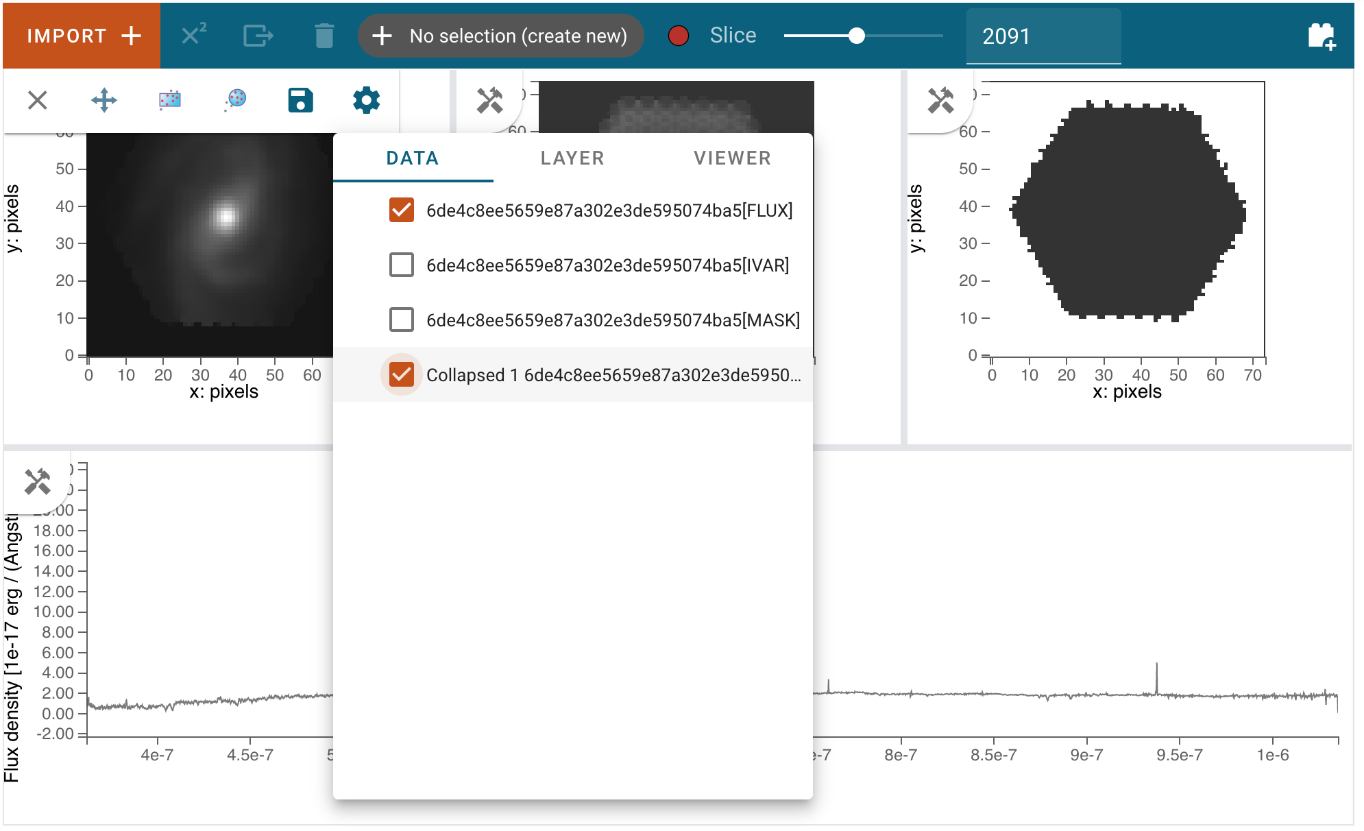
The Contours of a second image can also be plotted over a first image or cube. Add the second image as data in the data drop-down tab, and select both images. To visualize the contours of the second image, go to the Layer tab, select the layer to be contour-mapped, and set its Contour to be on and its Bitmap to be off. The contours of the second image will appear superimposed on the first image. In the second figure below, we show the contours of an image generated using the Collapse plugin plotted over leftmost cube viewer. If you overplot them on a cube, the contours will remain unchanged as you scrub through the cube.
Unit Conversion
See also
- Unit Conversion
Specviz documentation on unit conversion.
Line Lists
See also
- Line Lists
Specviz documentation on line lists.
Line Analysis
See also
- Line Analysis
Specviz documentation on line analysis.
Moment Maps
The Moment Maps plugin can be used to create a 2D image from a data cube. Mathematically, a moment is an integral of a 1D curve multiplied by the abscissa to some power. The plugin integrates the flux density along the spectral axis to compute a moment map. The order of the moment map (0, 1, 2, …) indicates the power-law index to which the spectral axis is raised. A ‘moment 0’ map gives the integrated flux over a spectral region. Similarly, ‘moment 1’ is the flux-weighted centroid (e.g. line center) and a ‘moment 2’ is the dispersion (e.g. wavelength or velocity dispersion) along the spectral axis. Moments 3 and 4 are less commonly utilized, but correspond to the skewness and kurtosis of a spectral feature.
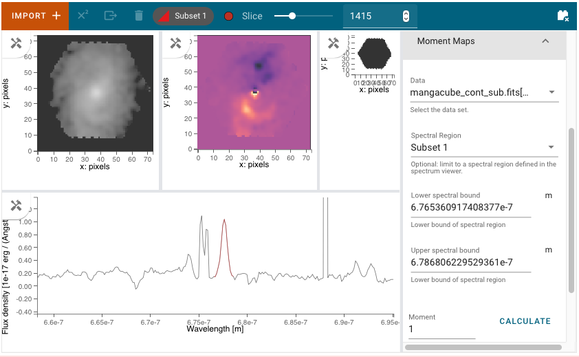
To make a moment map, first go to the Moment Maps plugin and select the cube dataset using the Data pulldown. To specify the spectral feature of interest, you can either create and select a Region in the spectrum viewer, or enter the lower and upper spectral bounds manually in the plugin. Next, enter the Moment index to specifiy the order of the moment map. When you press CALCULATE, a 2D moment map is created. You can load this into any image viewer pane to inspect the result. You can also save the result to a FITS format file by pressing SAVE AS FITS
For example, the middle image viewer in figure above shows the Moment 1 map for a continuum-subtracted cube. Note that the cube should first be continuum-subtracted in order to create continuum-free moment maps of an emission line. Moment maps of continuum emission can also be created, but moments other than moment 0 may not be physically meaningful. Also note that the units in the moment 1 and moment 2 maps reflect the units of the spectral axis (Angstroms in this case). The units of the input cube should first be converted to velocity units before running the plugin if those units are desired for the output moment maps.
Line or Continuum Maps
There are at least three ways to make a line map using one of three Cubeviz plugins: Collapse, Moment Maps, or Model Fitting. Line maps created using the first two methods require an input data cube that is already continuum-subtracted. Continuum maps can be created in a similar way for data that is not continuum-subtracted.
To make a line or continuum map using the Collapse plugin, first import a data cube into Cubeviz. Next, go to the Collapse plugin and select the input data using the Data pulldown. Then set the Axis to the wavelength axis (e.g. 0 for JWST data) and the method to ‘Sum’ (or any other desired method). Next either create and select a Region in the spectrum viewer, or enter the lower and upper spectral bounds manually. When you Apply the Collapse, a 2D image of the spectral region is created. You can load this line map in any image viewer pane to inspect the result.
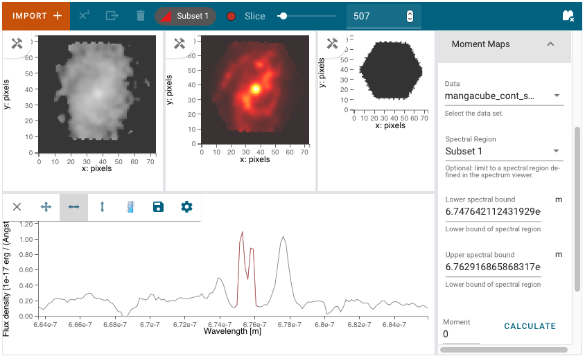
A line map can also be created using the Moment Maps Plugin using a similar workflow. Select the (continuum-subtracted) dataset in the Plugin using the Data pulldown. Then either select a subset in the Spectral Region pulldown or enter the lower and upper spectral bounds. Enter ‘0’ for Moment and press Calculate to create the moment 0 map. The resultant 2D image is the flux integral of the cube over the selected spectral region, and may be displayed in any image viewer, as shown in the middle image viewer in the figure above.
The third method to create a map is via the Model Fitting plugin. First create and fit a model (e.g. a Gaussian plus continuum model) to an individual spectrum. Next, fit this model to every spaxel in your data cube. The resultant model parameter cube can be retrieved in a notebook. The line or continuum flux in each spatial pixel can then be computed by integrating over the line or continuum spectral region of interest.