
Data Analysis Plugins#
Note
This is the config-specific version of documentation and is deprecated. See the general documentation for the most up-to-date information.
The Cubeviz data analysis plugins are meant to aid quick-look analysis of 2D image data, and both 1D and 3D spectroscopic data. All plugins are accessed via the plugin icon in the upper right corner of the Cubeviz application.
For spectroscopic data, functions can generally be applied to both 1D and 3D datasets,
represented as Spectrum objects.
Plugins that are specific to 1D spectra are described in
more detail under Specviz: Data Analysis Plugins.
In many cases, these capabilities can be further applied on a per-spaxel basis
within a cube.
Metadata Viewer#
See also
- Metadata Viewer
Documentation on using the metadata viewer.
Plot Options#
This plugin gives access to per-viewer and per-layer plotting options. To show axes on image viewers, toggle on the “Show axes” option at the bottom of the plugin.
See also
- Image Plot Options
Documentation on Imviz display settings in the Jdaviz viewers.
See also
- Spectral Plot Options
Documentation on Specviz display settings in the Jdaviz viewers.
Data Quality#
Visualize data quality arrays for spectral cubes from JWST.
See also
- Data Quality Plugin
Follow the link to the rest of the Data Quality plugin documentation.
Subset Tools#
See also
- Subset Tools
Imviz documentation describing the concept of subsets in Jdaviz.
Markers#
See also
- Markers
Imviz documentation describing the markers plugin.
Slice#
The slice plugin provides the ability to select the slice of the cube currently visible in the image viewers, with the corresponding wavelength highlighted in the spectrum viewer.
To choose a specific slice, enter an approximate wavelength (in which case the nearest slice will be selected and the wavelength entry will “span” to the exact value of that slice). The snapping behavior can be disabled in the plugin settings to allow for smooth scrubbing, in which case the closest slice will still be displayed in the cube viewer.
The spectrum viewer also contains a tool to allow clicking and dragging in the spectrum plot to choose the currently selected slice. When the slice tool is active, clicking anywhere on the spectrum viewer will select the nearest slice across all viewers, even if the indicator is off-screen.
For your convenience, there are also player-style buttons with the following functionality:
Jump to first
Previous slice
Play/Pause
Next slice
Jump to last
Gaussian Smooth#
Gaussian smoothing can be applied either to the spectral or spatial dimensions of a cube.
See also
- Gaussian Smooth
Specviz documentation on gaussian smoothing in the spectral dimension of 1D spectra.
Collapse#
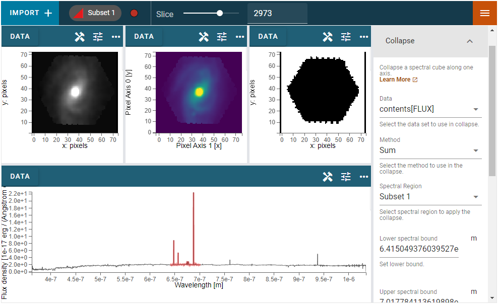
The Collapse plugin collapses a spectral cube along the wavelength axis to create a 2D spatial image. For spatial axes, the full extent of the selected dimension is included in the collapse. For the spectral axis, a wavelength range for collapse can be specified using a spectral subset or by entering the wavelength range manually.
To make a 2D image, first go to the Collapse plugin and select the cube dataset using the Data pulldown. Next, select the method for collapse (Mean, Median, Min, Max, or Sum) in the Method pulldown. To collapse a limited spectral subregion, you can either create and select a Region in the spectrum viewer, or enter the lower and upper spectral bounds manually. When you APPLY the Collapse, a 2D image is created. You can load this into any image viewer pane to inspect the result. For example, the Collapse Sum over an emission line is shown in the middle image viewer of the above figure.
Model Fitting#
See also
- Model Fitting
Specviz documentation on fitting spectral models.
For Cubeviz, there is an additional option to fit the model over each individual spaxel by enabling the Cube Fit toggle before pressing Fit Model. The best-fit parameters for each spaxel are stored in planes and saved in a data structure. The resulting model itself is saved with the label specified in the Output Data Label field.
See also
- Export Models
Documentation on exporting model fitting results.
Unit Conversion#
See also
- Unit Conversion
Specviz documentation on unit conversion.
Line Lists#
See also
- Line Lists
Specviz documentation on line lists.
Line Analysis#
See also
- Line Analysis
Specviz documentation on line analysis.
Currently the Line Analysis plugin in Cubeviz will calculate statistics for spectral features in the collapsed spectrum, which is visualized in the spectrum viewer. The propagation of uncertainties from the uncertainty cube to the collapsed spectrum is still work in progress. As a result, uncertainties generated by the Line Analysis plugin are not provided.
Moment Maps#
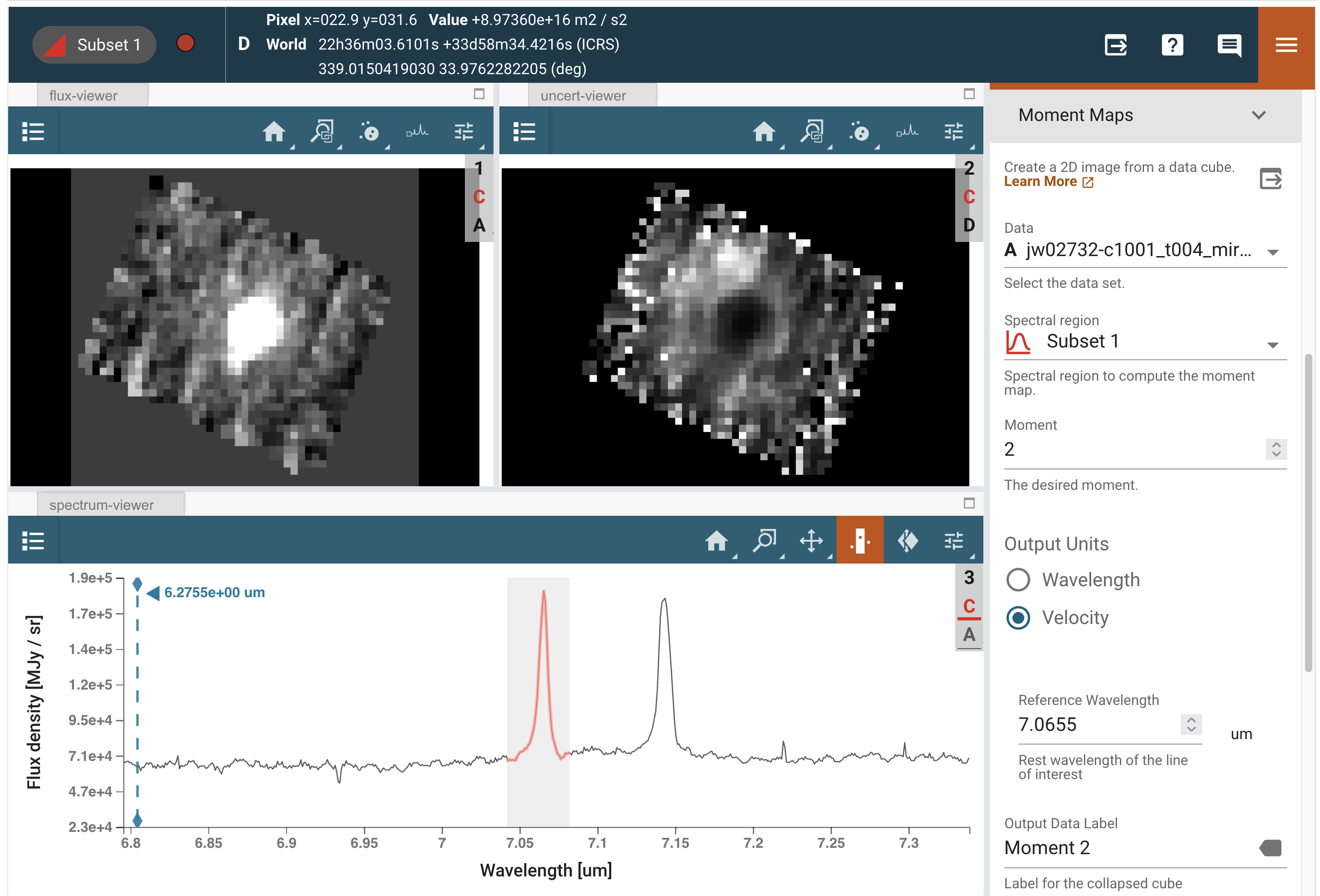
The Moment Maps plugin can be used to create a 2D image from a data cube. Mathematically, a moment is an integral of a 1D curve multiplied by the abscissa to some power. The plugin integrates the flux density along the spectral axis to compute a moment map. The order of the moment map (0, 1, 2, …) indicates the power-law index to which the spectral axis is raised. A ‘moment 0’ map gives the integrated flux over a spectral region. Similarly, ‘moment 1’ is the flux-weighted centroid (e.g., line center) and ‘moment 2’ is the dispersion (e.g., wavelength or velocity dispersion) along the spectral axis. Moments 3 and 4 are less commonly utilized, but correspond to the skewness and kurtosis of a spectral feature.
To make a moment map, first go to the Moment Maps plugin and select the cube dataset using the Data pulldown. To specify the spectral feature of interest, you can either create and select a Region in the spectrum viewer, or enter the lower and upper spectral bounds manually in the plugin. Next, enter the Moment index to specify the order of the moment map. When you press CALCULATE, a 2D moment map is created. You can load this into any image viewer pane to inspect the result. You can also save the result to a FITS format file by pressing SAVE AS FITS.
For example, the right image viewer in the screenshot above shows the Moment 2 map for a continuum-subtracted cube. Note that the cube should first be continuum-subtracted in order to create continuum-free moment maps of an emission line. Moment maps of continuum emission can also be created, but moments other than moment 0 may not be physically meaningful. Also note that by default, the units in the moment 1 and moment 2 maps reflect the units of the spectral axis (microns in this case). For moments higher than 0, the output units can instead be converted to velocity (e.g., m/s for moment 1, m2/s2 for moment 2, etc.) by selecting the Velocity radio button under Output Units and providing a reference wavelength, commonly that of the spectral line of interest.
Line or Continuum Maps#
There are at least three ways to make a line map using one of three Cubeviz plugins: Collapse, Moment Maps, or Model Fitting. Line maps created using the first two methods require an input data cube that is already continuum-subtracted. Continuum maps can be created in a similar way for data that is not continuum-subtracted.
To make a line or continuum map using the Collapse Plugin, first import a data cube into Cubeviz. Next, go to the Collapse plugin and select the input data using the Data pulldown. Then set the Axis to the wavelength axis (e.g. 0 for JWST data) and the method to ‘Sum’ (or any other desired method). Next either create and select a Region in the spectrum viewer, or enter the lower and upper spectral bounds manually. When you Apply the Collapse, a 2D image of the spectral region is created. You can load this line map in any image viewer pane to inspect the result.
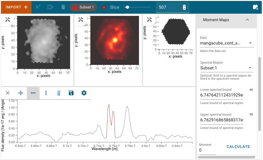
A line map can also be created using the Moment Maps Plugin using a similar workflow. Select the (continuum-subtracted) dataset in the Plugin using the Data pulldown. Then either select a subset in the Spectral Region pulldown or enter the lower and upper spectral bounds. Enter ‘0’ for Moment and press Calculate to create the moment 0 map. The resultant 2D image is the flux integral of the cube over the selected spectral region, and may be displayed in any image viewer, as shown in the middle image viewer in the figure above.
The third method to create a map is via the Model Fitting Plugin. First create and fit a model (e.g. a Gaussian plus continuum model) to an individual spectrum. Next, fit this model to every spaxel in your data cube. The resultant model parameter cube can be retrieved in a notebook. The line or continuum flux in each spatial pixel can then be computed by integrating over the line or continuum spectral region of interest.
3D Spectral Extraction#
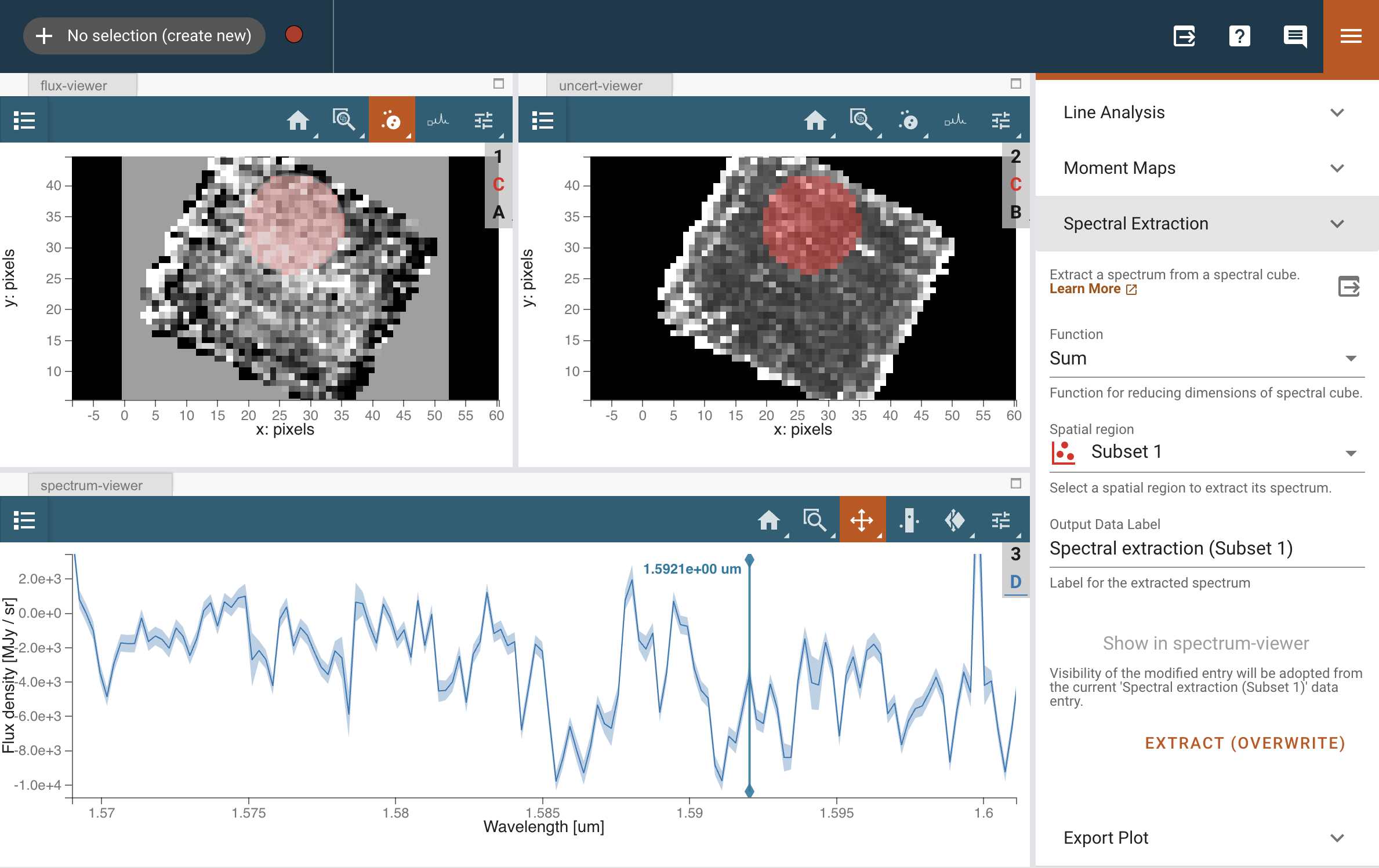
The 3D Spectral Extraction plugin produces a 1D spectrum from a spectral cube. The 1D spectrum can be computed via the sum, mean, minimum, or maximum of the spatial dimensions in the spectral cube. Select an extraction operation from the Function dropdown, and optionally choose a Spatial region, if you have one. Click EXTRACT to produce a new 1D spectrum dataset from the spectral cube, which has uncertainties propagated by astropy.nddata. By default, if a mask was loaded with the cube, it will be applied to the cube when extracting in addition to any subsets chosen as an aperture. This is not currently done for Data Quality arrays, e.g. the DQ extension in JWST files.
To interact with the plugin via the API in a notebook, access the plugin object via:
sp_ext = cubeviz.plugins['3D Spectral Extraction']
If using a simple subset (currently only works for a circular subset applied to data with spatial axis units in wavelength) for the spatial aperture, an option to make the aperture wavelength dependent will appear. If checked, this will create a cone aperture that increases linearly with wavelength. The formula for a circular aperture is (for other shapes, radius is replaced by appropriate shape attributes):
radii = ((all_wavelengths / reference_wavelength) *
    aperture.selected_spatial_region.radius)
The reference wavelength for the cone can be changed using the Adopt Current Slice button.
The method of aperture masking can also be changed using the Aperture masking method dropdown. To see a description for each of these options, please see Aperture and Pixel Overlap. Using the exact aperture method with the min or max functions is not supported.
Aperture Photometry#
Cubeviz allows aperture photometry on some 3D and 2D data, as long as they have valid flux units. For 3D data, the current Slice is used.
See also
- Imviz Aperture Photometry
Imviz documentation describing the concept of aperture photometry in Jdaviz.
Sonify Data#
This plugin uses the Strauss package to turn data cubes into audio grids (by pressing the Sonify Data button) that can be played while the mouse is hovering over the flux viewer. A range of the cube can be sonified by creating and selecting a spectral subset from the Spectral range dropdown and then pressing the Sonify Data button. The output device for sound can be changed by using the Sound device dropdown.
Once sonified, the resulting layers can be adjusted in the Plot Options plugin so that multiple sonified layers can be adjusted like a mixing board.
Note
For mac m-series users, the Strauss library requires the
sounddevice and
PortAudio libraries. In order to avoid errors with the sonification
process, sounddevice and PortAudio must be installed as follows (these steps can be followed
either before or after installing Strauss itself):
Download the latest/stable
PortAudiorelease from PortAudio’s website.Unpack the tarball and
cdinto theportaudiodirectory.Following the ‘debug’ build instructions, run
./configure --enable-mac-debug && make && sudo make install. This will place a “libportaudio.dylib” in the directory “usr/local/lib/” whichsounddevicewill link to.Install
sounddeviceviapip(notcondaascondawill attempt to install and link to it’s own portaudio).Install
Straussif not already done and proceed with the sonification.
Export#
This plugin offers the ability to export:
the plot in a given viewer as a PNG or SVG file,
a table in a plugin to ecsv,
image subsets (region) as a fits or reg file; spectral subsets as ecsv.
Movie#
Note
For MPEG-4, this feature needs opencv-python to be installed;
see opencv-python on PyPI.
Expand the “Export to video” section, then enter the desired starting and ending slice indices (inclusive), the frame rate in frames per second (FPS), and the filename. If a path is not given, the file will be saved to current working directory. Any existing file with the same name will be silently replaced.
When you are ready, click the Export to MP4 button. The movie will be recorded at the given FPS. While recording is in progress, it is highly recommended that you leave the app alone until it is done.
While recording, there is an option to interrupt the recording when something goes wrong (e.g., it is taking too long or you realized you entered the wrong inputs). Click on the stop icon next to the Export to MP4 button to interrupt it. Doing so will result in no output video.